|
Procedure
The program is proposed as a passive modular addition to supplement a program actively directing the robot’s motion. The agent will provide ease of availability to the raw data by passing a dynamic pointer to the array representing the occupancy grid. The main program may then direct the robot to transverse an exploratory or programmed path through the environment. The mapping agent is a background program that requires regular sensor updates to incrementally build a grid-map. When the main program starts it calls the mapping agent subprogram which sets the operating parameters and initializes the timer processes. The major modules are all cyclic work procedures and are named:
4.1 Incremental Mapping Module The Incremental Mapping module (IMM) builds the grid matrix and embodies the core of the proposed project. As can be seen in the top portion of Figure 3, the Incremental Mapping module requests information from the robot, processes the returned data and updates the dynamic representation in memory. Figure 3. The Incremental Mapping Module (IMM) Level 0 Data Flow Diagram 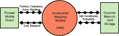
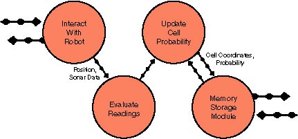
Level 1 Data Flow Diagram
|
Finally it times out for a pre-defined period and relinquishes control. Figure 3 also shows the major components of the IMM.
In the Interaction module, the data flow to the robot consists of requesting data on position, orientation and the individual sonar distance readings. Position of the robot is obtained using the functions paiRobotX() and paiRobotY(). Current heading is available through paiRobotHeading(). Spatial data is collected from each sonar with paiSonarRange(). In the Evaluate Readings module, the current pose is compared to the previous poses to determine if the sensor readings should be further processed. If the observation viewpoint is unchanged for the last several readings the module times out; otherwise the sonar readings are evaluated and used to update the occupancy-grid data.
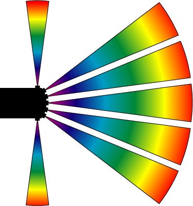
To understand the technique employed to evaluate the sonar data requires some understanding of the ultrasonic sensors. As shown in Figure 4, the Pioneer robot is equipped with a sonar array composed of seven emitter/receiver transducers. This array covers an arc of 180 degrees centered on the robot’s forward direction of movement. Each pinger will return the distance, measured in millimeters, to the closest object detected inside the zone of coverage. A transducer emits a short burst of 40kHz ultrasonic sound. It then waits a few milliseconds and then starts listening for an echo. As soon as a reflection of sufficient intensity is received, the circuitry will report an object detected. The sensitivity of the echo detection circuitry automatically increases, in steps, every few milliseconds as the ultrasound travels outward. This is to allow for weaker echoes from objects at greater distances. The consequence is that it becomes more vulnerable to spurious signals. If no object is detected, the value returned by the pai function is close to the maximum range; which is around 5 meters. The minimum range is around 0.2 meters.
Figure 4. The Robot Sonar Array
In the Interaction module, the data flow to the robot consists of requesting data on position, orientation and the individual sonar distance readings. Position of the robot is obtained using the functions paiRobotX() and paiRobotY(). Current heading is available through paiRobotHeading(). Spatial data is collected from each sonar with paiSonarRange(). In the Evaluate Readings module, the current pose is compared to the previous poses to determine if the sensor readings should be further processed. If the observation viewpoint is unchanged for the last several readings the module times out; otherwise the sonar readings are evaluated and used to update the occupancy-grid data.
To understand the technique employed to evaluate the sonar data requires some understanding of the ultrasonic sensors. As shown in Figure 4, the Pioneer robot is equipped with a sonar array composed of seven emitter/receiver transducers. This array covers an arc of 180 degrees centered on the robot’s forward direction of movement. Each pinger will return the distance, measured in millimeters, to the closest object detected inside the zone of coverage. A transducer emits a short burst of 40kHz ultrasonic sound. It then waits a few milliseconds and then starts listening for an echo. As soon as a reflection of sufficient intensity is received, the circuitry will report an object detected. The sensitivity of the echo detection circuitry automatically increases, in steps, every few milliseconds as the ultrasound travels outward. This is to allow for weaker echoes from objects at greater distances. The consequence is that it becomes more vulnerable to spurious signals. If no object is detected, the value returned by the pai function is close to the maximum range; which is around 5 meters. The minimum range is around 0.2 meters.
Figure 4. The Robot Sonar Array
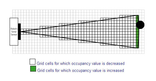
The module that processes the sonar data is titled Evaluate Readings. Input for the module consists of robot pose and the various sonar readings. Output to the update module is a cell coordinate with the new cell update. The returned value for each sensor is processed in one of the following manners:
- If the returned value is close to the maximum value, it is assumed that the sensor has detected no obstacles in any of the grid locations within the footprint of that sensor. All of these grid locations have their occupation probability reduced.
- If the value is less than a predefined threshold limit, the grid location(s) that correspond to the returned distance have their occupation probability incremented. Additionally all of the grid locations from the robot to the obstacle have their occupational probability decreased.
Figure 5. Illustration of Occupancy Value Changes as Obstacles are Encountered
The statistical methods for calculating the cell probability should take into account all of the prior readings for each cell. Storing these measurements for future evaluations entails a large cost both in memory and time. Any method employed should use the minimum number of values necessary to achieve accurate results. Ideally, the method would only require the retention of previous probability and the new update reading to arrive at the new cell probability. This keeps storage overhead at a minimum.
Upon initialization a cell is given the probability of 0.5 which represents an ambiguous probability of occupancy. A value of 1 represents the highest value of probability that the cell is occupied and a value of 0 represents maximum probability that the cell is unoccupied. The simplest technique to manipulate the cells is to increment or decrement the cell’s probability by a constant amount each time a new sensor reading is taken. The set amount can be adjusted depending upon factors such as sensor reliability and average number of cell readings. The drawback to this method is that the probabilities linearly approach the limit values and require quite a few measurements to do so. Increasing the step amount corrects this problem but makes the method more sensitive to sensor noise. Most methods employed use some form of Bayesian statistical analysis. Bayesian Forecasting requires that the noise signal follow a random normal distribution. The Bayesian approach yields a response that resembles an exponential curve. Figure 6 shows that just a couple of readings cause the probability to rapidly jump toward one of the absolute values yet approach it like an exponential curve. By manipulating the update values the rate of approach can be adjusted as needed.
Figure 6. Rates of Probability Update
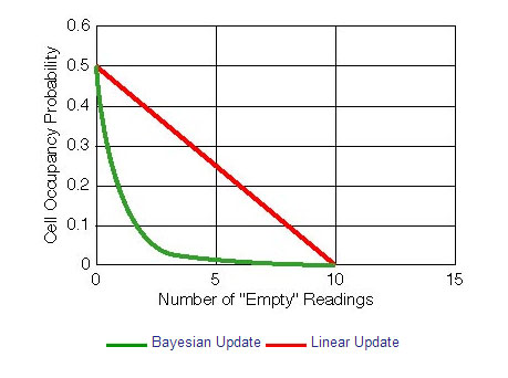
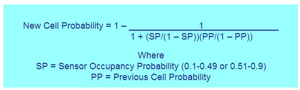
Both methods will be implemented to determine relative efficacy. The linear method offers simplicity and the Bayesian method yields better statistical probabilities. The equation that is proposed for the Bayesian method is:
In Figure 6, the Bayesian Update is using 0.3 as the value of the Sensor Occupancy Probability (SP) for all of the readings and the initialization probability is 0.5.
The function of the Update Cell Probability module is very direct. It receives the cell coordinates and sensor probability from the Evaluate Readings module. It then requests the cell’s current probability from the Memory Storage module. Using this data it determines the updated cell value and submits the new probability for storage.
The occupancy grid for this project is a two-dimensional matrix that represents the mapping area. It requires being able to index the array in a Cartesian-coordinate style. Each cell of the array must store the grid coordinates and a floating-point number between 0 and 1. To enable the easy transfer of the occupancy grid mapping data, the array should be addressable by an index pointer. Alternately the matrix can be static or dynamically created as needed using a chain and bucket method of node construction. In Figure 7 the buckets can represent the Y-axis with the chains forming the X-elements.
Figure 7. Dynamic Memory Structure
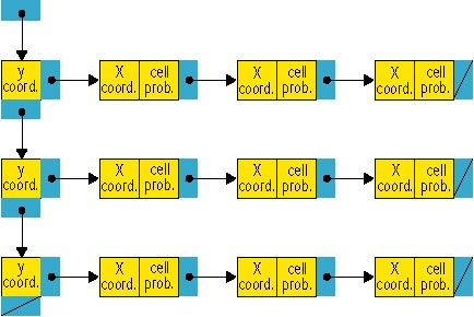
The bucket nodes will have the Y-coordinate value and pointers to previous and next Y-coordinate and to the lowest X-node with this Y-coordinate. All the X-nodes tied to this bucket share the Y-value and are in sorted order. The X-nodes will store the probability for the cell and the X-coordinate value.
The Memory Storage module is in charge of creating, organizing and accessing the occupancy grid memory locations. It performs three main functions:
4.2 Mapping Display Module
The Mapping Display module is a timed procedure that is optionally executed. The module will be an X-Windows based GUI application that displays the grid map. Initially the program scans the matrix to establish the absolute dimensions of the map. It will use a pixmap to store the display drawing. The process calls each cell in the array, reads the probability of that cell and draws the representation of that cell into the pixmap. When it completes the cells, the scales and axes are inserted followed by the legend. After the pixmap is completed, it is copied into the active display. The process times out and repeats the process after the delay period. The module has a scrollbar as an adjusting method to set the sensitivity guidelines for converting the probabilities into drawings.
4.3 Hardcopy Module
The Hardcopy module will transcribe the accumulated spatial data into a file stored in non-volatile memory. This process is cyclically performed to store the updates and keep the stored file current with the information stored in the memory array. In simple form, the file is a list of data structures comprised of X-coordinate, Y-coordinate and probability. The cycle time is not critical and is determined by factors such as the robustness of the program and the duration of the robot's main program. Primarily the module should execute frequently enough that a crash would not cause a loss of a significant portion of the accumulated data.
The Memory Storage module is in charge of creating, organizing and accessing the occupancy grid memory locations. It performs three main functions:
- Retrieve the current occupational grid probability value of an addressable cell.
- Store an occupational grid probability value in an addressable cell.
- Create new cells, initialize them to a probability of 0.5 and tie them into the matrix.
4.2 Mapping Display Module
The Mapping Display module is a timed procedure that is optionally executed. The module will be an X-Windows based GUI application that displays the grid map. Initially the program scans the matrix to establish the absolute dimensions of the map. It will use a pixmap to store the display drawing. The process calls each cell in the array, reads the probability of that cell and draws the representation of that cell into the pixmap. When it completes the cells, the scales and axes are inserted followed by the legend. After the pixmap is completed, it is copied into the active display. The process times out and repeats the process after the delay period. The module has a scrollbar as an adjusting method to set the sensitivity guidelines for converting the probabilities into drawings.
4.3 Hardcopy Module
The Hardcopy module will transcribe the accumulated spatial data into a file stored in non-volatile memory. This process is cyclically performed to store the updates and keep the stored file current with the information stored in the memory array. In simple form, the file is a list of data structures comprised of X-coordinate, Y-coordinate and probability. The cycle time is not critical and is determined by factors such as the robustness of the program and the duration of the robot's main program. Primarily the module should execute frequently enough that a crash would not cause a loss of a significant portion of the accumulated data.
